Code vectorization¶

Contents

Introduction ¶

Code vectorization means that the problem you’re trying to solve is inherently vectorizable and only requires a few NumPy tricks to make it faster. Of course it does not mean it is easy or straightforward, but at least it does not necessitate totally rethinking your problem (as it will be the case in the `Problem vectorization`_ chapter). Still, it may require some experience to see where code can be vectorized. Let’s illustrate this through a simple example where we want to sum up two lists of integers. One simple way using pure Python is:

def add_python(Z1,Z2):
    return [z1+z2 for (z1,z2) in zip(Z1,Z2)]

This first naive solution can be vectorized very easily using NumPy:

def add_numpy(Z1,Z2):
    return np.add(Z1,Z2)

Without any surprise, benchmarking the two approaches shows the second method is the fastest with one order of magnitude.

>>> Z1 = random.sample(range(1000), 100)
>>> Z2 = random.sample(range(1000), 100)
>>> timeit("add_python(Z1, Z2)", globals())
1000 loops, best of 3: 68 usec per loop
>>> timeit("add_numpy(Z1, Z2)", globals())
10000 loops, best of 3: 1.14 usec per loop

Not only is the second approach faster, but it also naturally adapts to the shape of Z1 and Z2. This is the reason why we did not write Z1 + Z2 because it would not work if Z1 and Z2 were both lists. In the first Python method, the inner + is interpreted differently depending on the nature of the two objects such that if we consider two nested lists, we get the following outputs:

>>> Z1 = [[1, 2], [3, 4]]
>>> Z2 = [[5, 6], [7, 8]]
>>> Z1 + Z2
[[1, 2], [3, 4], [5, 6], [7, 8]]
>>> add_python(Z1, Z2)
[[1, 2, 5, 6], [3, 4, 7, 8]]
>>> add_numpy(Z1, Z2)
[[ 6  8]
 [10 12]]

The first method concatenates the two lists together, the second method concatenates the internal lists together and the last one computes what is (numerically) expected. As an exercise, you can rewrite the Python version such that it accepts nested lists of any depth.

Uniform vectorization ¶

Uniform vectorization is the simplest form of vectorization where all the elements share the same computation at every time step with no specific processing for any element. One stereotypical case is the Game of Life that has been invented by John Conway (see below) and is one of the earliest examples of cellular automata. Those cellular automata can be conveniently regarded as an array of cells that are connected together with the notion of neighbours and their vectorization is straightforward. Let me first define the game and we’ll see how to vectorize it.

Figure 4.1

Conus textile snail exhibits a cellular automaton pattern on its shell. Image by Richard Ling, 2005.

The Game of Life ¶

Note

Excerpt from the Wikipedia entry on the Game of Life

The Game of Life is a cellular automaton devised by the British mathematician John Horton Conway in 1970. It is the best-known example of a cellular automaton. The “game” is actually a zero-player game, meaning that its evolution is determined by its initial state, needing no input from human players. One interacts with the Game of Life by creating an initial configuration and observing how it evolves.

The universe of the Game of Life is an infinite two-dimensional orthogonal grid of square cells, each of which is in one of two possible states, live or dead. Every cell interacts with its eight neighbours, which are the cells that are directly horizontally, vertically, or diagonally adjacent. At each step in time, the following transitions occur:

Any live cell with fewer than two live neighbours dies, as if by underpopulation.
Any live cell with more than three live neighbours dies, as if by overcrowding.
Any live cell with two or three live neighbours lives, unchanged, to the next generation.
Any dead cell with exactly three live neighbours becomes a live cell.

The initial pattern constitutes the ‘seed’ of the system. The first generation is created by applying the above rules simultaneously to every cell in the seed – births and deaths happen simultaneously, and the discrete moment at which this happens is sometimes called a tick. (In other words, each generation is a pure function of the one before.) The rules continue to be applied repeatedly to create further generations.

Python implementation ¶

Note

We could have used the more efficient python array interface but it is more convenient to use the familiar list object.

In pure Python, we can code the Game of Life using a list of lists representing the board where cells are supposed to evolve. Such a board will be equipped with border of 0 that allows to accelerate things a bit by avoiding having specific tests for borders when counting the number of neighbours.

Z = [[0,0,0,0,0,0],
     [0,0,0,1,0,0],
     [0,1,0,1,0,0],
     [0,0,1,1,0,0],
     [0,0,0,0,0,0],
     [0,0,0,0,0,0]]

Taking the border into account, counting neighbours then is straightforward:

def compute_neighbours(Z):
    shape = len(Z), len(Z[0])
    N  = [[0,]*(shape[1]) for i in range(shape[0])]
    for x in range(1,shape[0]-1):
        for y in range(1,shape[1]-1):
            N[x][y] = Z[x-1][y-1]+Z[x][y-1]+Z[x+1][y-1] \
                    + Z[x-1][y]            +Z[x+1][y]   \
                    + Z[x-1][y+1]+Z[x][y+1]+Z[x+1][y+1]
    return N

To iterate one step in time, we then simply count the number of neighbours for each internal cell and we update the whole board according to the four aforementioned rules:

def iterate(Z):
    N = compute_neighbours(Z)
    for x in range(1,shape[0]-1):
        for y in range(1,shape[1]-1):
             if Z[x][y] == 1 and (N[x][y] < 2 or N[x][y] > 3):
                 Z[x][y] = 0
             elif Z[x][y] == 0 and N[x][y] == 3:
                 Z[x][y] = 1
    return Z

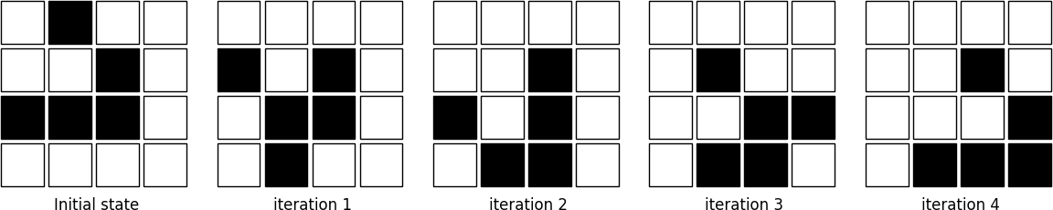
The figure below shows four iterations on a 4x4 area where the initial state is a glider, a structure discovered by Richard K. Guy in 1970.

Figure 4.2

The glider pattern is known to replicate itself one step diagonally in 4 iterations.

NumPy implementation ¶

Starting from the Python version, the vectorization of the Game of Life requires two parts, one responsible for counting the neighbours and one responsible for enforcing the rules. Neighbour-counting is relatively easy if we remember we took care of adding a null border around the arena. By considering partial views of the arena we can actually access neighbours quite intuitively as illustrated below for the one-dimensional case:

               ┏━━━┳━━━┳━━━┓───┬───┐
        Z[:-2] ┃ 0 ┃ 1 ┃ 1 ┃ 1 │ 0 │ (left neighbours)
               ┗━━━┻━━━┻━━━┛───┴───┘
                     ↓︎
           ┌───┏━━━┳━━━┳━━━┓───┐
   Z[1:-1] │ 0 ┃ 1 ┃ 1 ┃ 1 ┃ 0 │ (actual cells)
           └───┗━━━┻━━━┻━━━┛───┘
                     ↑
       ┌───┬───┏━━━┳━━━┳━━━┓
Z[+2:] │ 0 │ 1 ┃ 1 ┃ 1 ┃ 0 ┃ (right neighbours)
       └───┴───┗━━━┻━━━┻━━━┛

Going to the two dimensional case requires just a bit of arithmetic to make sure to consider all the eight neighbours.

N = np.zeros(Z.shape, dtype=int)
N[1:-1,1:-1] += (Z[ :-2, :-2] + Z[ :-2,1:-1] + Z[ :-2,2:] +
                 Z[1:-1, :-2]                + Z[1:-1,2:] +
                 Z[2:  , :-2] + Z[2:  ,1:-1] + Z[2:  ,2:])

For the rule enforcement, we can write a first version using NumPy’s argwhere method that will give us the indices where a given condition is True.

# Flatten arrays
N_ = N.ravel()
Z_ = Z.ravel()

# Apply rules
R1 = np.argwhere( (Z_==1) & (N_ < 2) )
R2 = np.argwhere( (Z_==1) & (N_ > 3) )
R3 = np.argwhere( (Z_==1) & ((N_==2) | (N_==3)) )
R4 = np.argwhere( (Z_==0) & (N_==3) )

# Set new values
Z_[R1] = 0
Z_[R2] = 0
Z_[R3] = Z_[R3]
Z_[R4] = 1

# Make sure borders stay null
Z[0,:] = Z[-1,:] = Z[:,0] = Z[:,-1] = 0

Even if this first version does not use nested loops, it is far from optimal because of the use of the four argwhere calls that may be quite slow. We can instead factorize the rules into cells that will survive (stay at 1) and cells that will give birth. For doing this, we can take advantage of NumPy boolean capability and write quite naturally:

Note

We did not write Z = 0 as this would simply assign the value 0 to Z that would then become a simple scalar.

birth = (N==3)[1:-1,1:-1] & (Z[1:-1,1:-1]==0)
survive = ((N==2) | (N==3))[1:-1,1:-1] & (Z[1:-1,1:-1]==1)
Z[...] = 0
Z[1:-1,1:-1][birth | survive] = 1

If you look at the birth and survive lines, you’ll see that these two variables are arrays that can be used to set Z values to 1 after having cleared it.

Figure 4.3

The Game of Life. Gray levels indicate how much a cell has been active in the past.

Exercise ¶

Reaction and diffusion of chemical species can produce a variety of patterns, reminiscent of those often seen in nature. The Gray-Scott equations model such a reaction. For more information on this chemical system see the article Complex Patterns in a Simple System (John E. Pearson, Science, Volume 261, 1993). Let’s consider two chemical species $U$ and $V$ with respective concentrations $u$ and $v$ and diffusion rates $Du$ and $Dv$. $V$ is converted into $P$ with a rate of conversion $k$. $f$ represents the rate of the process that feeds $U$ and drains $U$, $V$ and $P$. This can be written as:

Chemical reaction	Equations
$U + 2V \rightarrow 3V$	$\dot{u} = Du \nabla^2 u - uv^2 + f(1-u)$
$V \rightarrow P$	$\dot{v} = Dv \nabla^2 v + uv^2 - (f+k)v$

Based on the Game of Life example, try to implement such reaction-diffusion system. Here is a set of interesting parameters to test:

Name	Du	Dv	f	k
Bacteria 1	0.16	0.08	0.035	0.065
Bacteria 2	0.14	0.06	0.035	0.065
Coral	0.16	0.08	0.060	0.062
Fingerprint	0.19	0.05	0.060	0.062
Spirals	0.10	0.10	0.018	0.050
Spirals Dense	0.12	0.08	0.020	0.050
Spirals Fast	0.10	0.16	0.020	0.050
Unstable	0.16	0.08	0.020	0.055
Worms 1	0.16	0.08	0.050	0.065
Worms 2	0.16	0.08	0.054	0.063
Zebrafish	0.16	0.08	0.035	0.060

The figure below shows some animations of the model for a specific set of parameters.

Figure 4.4

Reaction-diffusion Gray-Scott model. From left to right, Bacteria 1, Coral and Spiral Dense.

Sources ¶

game_of_life_python.py
game_of_life_numpy.py
gray_scott.py (solution to the exercise)

References ¶

John Conway new solitaire game “life”, Martin Gardner, Scientific American 223, 1970.
Gray Scott Model of Reaction Diffusion, Abelson, Adams, Coore, Hanson, Nagpal, Sussman, 1997.
Reaction-Diffusion by the Gray-Scott Model, Robert P. Munafo, 1996.

Temporal vectorization ¶

The Mandelbrot set is the set of complex numbers $c$ for which the function $f_c(z) = z^2+ c$ does not diverge when iterated from $z=0$, i.e., for which the sequence $f_c(0), f_c(f_c(0))$, etc., remains bounded in absolute value. It is very easy to compute, but it can take a very long time because you need to ensure a given number does not diverge. This is generally done by iterating the computation up to a maximum number of iterations, after which, if the number is still within some bounds, it is considered non-divergent. Of course, the more iterations you do, the more precision you get.

Figure 4.5

Romanesco broccoli, showing self-similar form approximating a natural fractal. Image by Jon Sullivan, 2004.

Python implementation ¶

A pure python implementation is written as:

def mandelbrot_python(xmin, xmax, ymin, ymax, xn, yn, maxiter, horizon=2.0):
    def mandelbrot(z, maxiter):
        c = z
        for n in range(maxiter):
            if abs(z) > horizon:
                return n
            z = z*z + c
        return maxiter
    r1 = [xmin+i*(xmax-xmin)/xn for i in range(xn)]
    r2 = [ymin+i*(ymax-ymin)/yn for i in range(yn)]
    return [mandelbrot(complex(r, i),maxiter) for r in r1 for i in r2]

The interesting (and slow) part of this code is the mandelbrot function that actually computes the sequence $f_c(f_c(f_c ...)))$. The vectorization of such code is not totally straightforward because the internal return implies a differential processing of the element. Once it has diverged, we don’t need to iterate any more and we can safely return the iteration count at divergence. The problem is to then do the same in NumPy. But how?

NumPy implementation ¶

The trick is to search at each iteration values that have not yet diverged and update relevant information for these values and only these values. Because we start from $Z = 0$, we know that each value will be updated at least once (when they’re equal to $0$, they have not yet diverged) and will stop being updated as soon as they’ve diverged. To do that, we’ll use NumPy fancy indexing with the less(x1,x2) function that return the truth value of (x1 < x2) element-wise.

def mandelbrot_numpy(xmin, xmax, ymin, ymax, xn, yn, maxiter, horizon=2.0):
    X = np.linspace(xmin, xmax, xn, dtype=np.float32)
    Y = np.linspace(ymin, ymax, yn, dtype=np.float32)
    C = X + Y[:,None]*1j
    N = np.zeros(C.shape, dtype=int)
    Z = np.zeros(C.shape, np.complex64)
    for n in range(maxiter):
        I = np.less(abs(Z), horizon)
        N[I] = n
        Z[I] = Z[I]**2 + C[I]
    N[N == maxiter-1] = 0
    return Z, N

Here is the benchmark:

>>> xmin, xmax, xn = -2.25, +0.75, int(3000/3)
>>> ymin, ymax, yn = -1.25, +1.25, int(2500/3)
>>> maxiter = 200
>>> timeit("mandelbrot_python(xmin, xmax, ymin, ymax, xn, yn, maxiter)", globals())
1 loops, best of 3: 6.1 sec per loop
>>> timeit("mandelbrot_numpy(xmin, xmax, ymin, ymax, xn, yn, maxiter)", globals())
1 loops, best of 3: 1.15 sec per loop

Faster NumPy implementation ¶

The gain is roughly a 5x factor, not as much as we could have expected. Part of the problem is that the np.less function implies $xn \times yn$ tests at every iteration while we know that some values have already diverged. Even if these tests are performed at the C level (through NumPy), the cost is nonetheless significant. Another approach proposed by Dan Goodman is to work on a dynamic array at each iteration that stores only the points which have not yet diverged. It requires more lines but the result is faster and leads to a 10x factor speed improvement compared to the Python version.

def mandelbrot_numpy_2(xmin, xmax, ymin, ymax, xn, yn, itermax, horizon=2.0):
    Xi, Yi = np.mgrid[0:xn, 0:yn]
    Xi, Yi = Xi.astype(np.uint32), Yi.astype(np.uint32)
    X = np.linspace(xmin, xmax, xn, dtype=np.float32)[Xi]
    Y = np.linspace(ymin, ymax, yn, dtype=np.float32)[Yi]
    C = X + Y*1j
    N_ = np.zeros(C.shape, dtype=np.uint32)
    Z_ = np.zeros(C.shape, dtype=np.complex64)
    Xi.shape = Yi.shape = C.shape = xn*yn

    Z = np.zeros(C.shape, np.complex64)
    for i in range(itermax):
        if not len(Z): break

        # Compute for relevant points only
        np.multiply(Z, Z, Z)
        np.add(Z, C, Z)

        # Failed convergence
        I = abs(Z) > horizon
        N_[Xi[I], Yi[I]] = i+1
        Z_[Xi[I], Yi[I]] = Z[I]

        # Keep going with those who have not diverged yet
        np.negative(I,I)
        Z = Z[I]
        Xi, Yi = Xi[I], Yi[I]
        C = C[I]
    return Z_.T, N_.T

The benchmark gives us:

>>> timeit("mandelbrot_numpy_2(xmin, xmax, ymin, ymax, xn, yn, maxiter)", globals())
1 loops, best of 3: 510 msec per loop

Visualization ¶

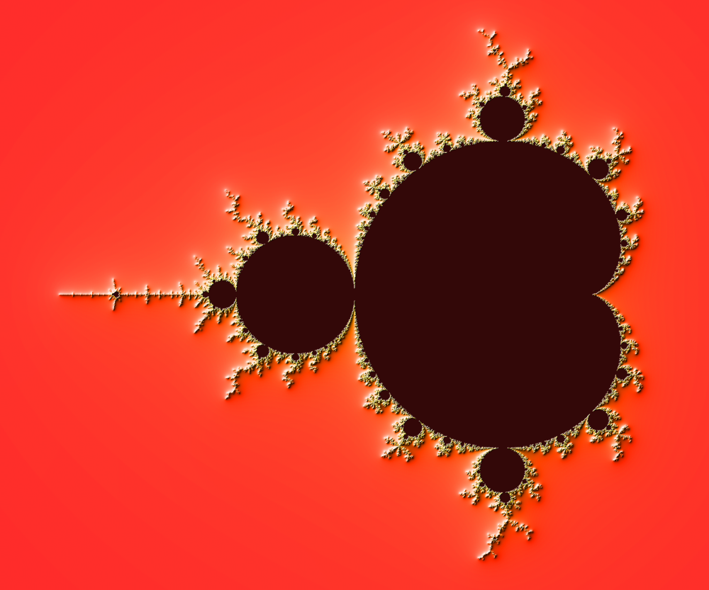
In order to visualize our results, we could directly display the N array using the matplotlib imshow command, but this would result in a “banded” image that is a known consequence of the escape count algorithm that we’ve been using. Such banding can be eliminated by using a fractional escape count. This can be done by measuring how far the iterated point landed outside of the escape cutoff. See the reference below about the renormalization of the escape count. Here is a picture of the result where we use recount normalization, and added a power normalized color map (gamma=0.3) as well as light shading.

Figure 4.6

The Mandelbrot as rendered by matplotlib using recount normalization, power normalized color map (gamma=0.3) and light shading.

Exercise ¶

Note

You should look at the ufunc.reduceat method that performs a (local) reduce with specified slices over a single axis.

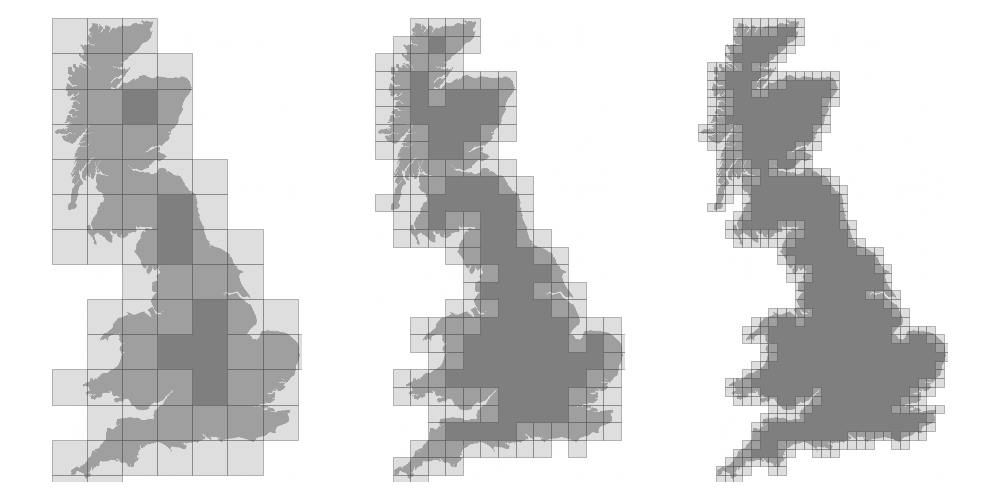
We now want to measure the fractal dimension of the Mandelbrot set using the Minkowski–Bouligand dimension. To do that, we need to do box-counting with a decreasing box size (see figure below). As you can imagine, we cannot use pure Python because it would be way too slow. The goal of the exercise is to write a function using NumPy that takes a two-dimensional float array and returns the dimension. We’ll consider values in the array to be normalized (i.e. all values are between 0 and 1).

Figure 4.7

The Minkowski–Bouligand dimension of the Great Britain coastlines is approximately 1.24.

$_images/fractal-dimension.png$

Sources ¶

mandelbrot.py
mandelbrot_python.py
mandelbrot_numpy_1.py
mandelbrot_numpy_2.py
fractal_dimension.py (solution to the exercise)

References ¶

How To Quickly Compute the Mandelbrot Set in Python, Jean Francois Puget, 2015.
My Christmas Gift: Mandelbrot Set Computation In Python, Jean Francois Puget, 2015.
Fast fractals with Python and NumPy, Dan Goodman, 2009.
Renormalizing the Mandelbrot Escape, Linas Vepstas, 1997.

Spatial vectorization ¶

Spatial vectorization refers to a situation where elements share the same computation but are in interaction with only a subgroup of other elements. This was already the case for the game of life example, but in some situations there is an added difficulty because the subgroup is dynamic and needs to be updated at each iteration. This the case, for example, in particle systems where particles interact mostly with local neighbours. This is also the case for “boids” that simulate flocking behaviors.

Figure 4.8

Flocking birds are an example of self-organization in biology. Image by Christoffer A Rasmussen, 2012.

Boids ¶

Note

Excerpt from the Wikipedia entry Boids

Boids is an artificial life program, developed by Craig Reynolds in 1986, which simulates the flocking behaviour of birds. The name “boid” corresponds to a shortened version of “bird-oid object”, which refers to a bird-like object.

As with most artificial life simulations, Boids is an example of emergent behavior; that is, the complexity of Boids arises from the interaction of individual agents (the boids, in this case) adhering to a set of simple rules. The rules applied in the simplest Boids world are as follows:

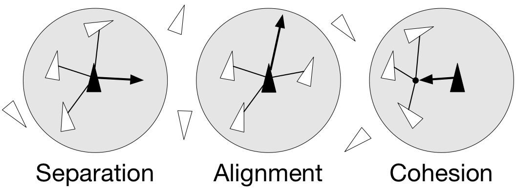
separation: steer to avoid crowding local flock-mates
alignment: steer towards the average heading of local flock-mates
cohesion: steer to move toward the average position (center of mass) of local flock-mates

Figure 4.9

Boids are governed by a set of three local rules (separation, cohesion and alignment) that serve as computing velocity and acceleration.

Python implementation ¶

Since each boid is an autonomous entity with several properties such as position and velocity, it seems natural to start by writing a Boid class:

import math
import random
from vec2 import vec2

class Boid:
    def __init__(self, x=0, y=0):
        self.position = vec2(x, y)
        angle = random.uniform(0, 2*math.pi)
        self.velocity = vec2(math.cos(angle), math.sin(angle))
        self.acceleration = vec2(0, 0)

The vec2 object is a very simple class that handles all common vector operations with 2 components. It will save us some writing in the main Boid class. Note that there are some vector packages in the Python Package Index, but that would be overkill for such a simple example.

Boid is a difficult case for regular Python because a boid has interaction with local neighbours. However, and because boids are moving, to find such local neighbours requires computing at each time step the distance to each and every other boid in order to sort those which are in a given interaction radius. The prototypical way of writing the three rules is thus something like:

def separation(self, boids):
    count = 0
    for other in boids:
        d = (self.position - other.position).length()
        if 0 < d < desired_separation:
            count += 1
            ...
    if count > 0:
        ...

 def alignment(self, boids): ...
 def cohesion(self, boids): ...

Full sources are given in the references section below, it would be too long to describe it here and there is no real difficulty.

To complete the picture, we can also create a Flock object:

class Flock:
    def __init__(self, count=150):
        self.boids = []
        for i in range(count):
            boid = Boid()
            self.boids.append(boid)

    def run(self):
        for boid in self.boids:
            boid.run(self.boids)

Using this approach, we can have up to 50 boids until the computation time becomes too slow for a smooth animation. As you may have guessed, we can do much better using NumPy, but let me first point out the main problem with this Python implementation. If you look at the code, you will certainly notice there is a lot of redundancy. More precisely, we do not exploit the fact that the Euclidean distance is reflexive, that is, $|x-y| = |y-x|$. In this naive Python implementation, each rule (function) computes $n^2$ distances while $\frac{n^2}{2}$ would be sufficient if properly cached. Furthermore, each rule re-computes every distance without caching the result for the other functions. In the end, we are computing $3n^2$ distances instead of $\frac{n^2}{2}$.

NumPy implementation ¶

As you might expect, the NumPy implementation takes a different approach and we’ll gather all our boids into a position array and a velocity array:

n = 500
velocity = np.zeros((n, 2), dtype=np.float32)
position = np.zeros((n, 2), dtype=np.float32)

The first step is to compute the local neighborhood for all boids, and for this we need to compute all paired distances:

dx = np.subtract.outer(position[:, 0], position[:, 0])
dy = np.subtract.outer(position[:, 1], position[:, 1])
distance = np.hypot(dx, dy)

We could have used the scipy cdist but we’ll need the dx and dy arrays later. Once those have been computed, it is faster to use the hypot method. Note that distance shape is (n, n) and each line relates to one boid, i.e. each line gives the distance to all other boids (including self).

From theses distances, we can now compute the local neighborhood for each of the three rules, taking advantage of the fact that we can mix them together. We can actually compute a mask for distances that are strictly positive (i.e. have no self-interaction) and multiply it with other distance masks.

Note

If we suppose that boids cannot occupy the same position, how can you compute mask_0 more efficiently?

mask_0 = (distance > 0)
mask_1 = (distance < 25)
mask_2 = (distance < 50)
mask_1 *= mask_0
mask_2 *= mask_0
mask_3 = mask_2

Then, we compute the number of neighbours within the given radius and we ensure it is at least 1 to avoid division by zero.

mask_1_count = np.maximum(mask_1.sum(axis=1), 1)
mask_2_count = np.maximum(mask_2.sum(axis=1), 1)
mask_3_count = mask_2_count

We’re ready to write our three rules:

Alignment

# Compute the average velocity of local neighbours
target = np.dot(mask, velocity)/count.reshape(n, 1)

# Normalize the result
norm = np.sqrt((target*target).sum(axis=1)).reshape(n, 1)
np.divide(target, norm, out=target, where=norm != 0)

# Alignment at constant speed
target *= max_velocity

# Compute the resulting steering
alignment = target - velocity

Cohesion

# Compute the gravity center of local neighbours
center = np.dot(mask, position)/count.reshape(n, 1)

# Compute direction toward the center
target = center - position

# Normalize the result
norm = np.sqrt((target*target).sum(axis=1)).reshape(n, 1)
np.divide(target, norm, out=target, where=norm != 0)

# Cohesion at constant speed (max_velocity)
target *= max_velocity

# Compute the resulting steering
cohesion = target - velocity

Separation

# Compute the repulsion force from local neighbours
repulsion = np.dstack((dx, dy))

# Force is inversely proportional to the distance
np.divide(repulsion, distance.reshape(n, n, 1)**2, out=repulsion,
          where=distance.reshape(n, n, 1) != 0)

# Compute direction away from others
target = (repulsion*mask.reshape(n, n, 1)).sum(axis=1)/count.reshape(n, 1)

# Normalize the result
norm = np.sqrt((target*target).sum(axis=1)).reshape(n, 1)
np.divide(target, norm, out=target, where=norm != 0)

# Separation at constant speed (max_velocity)
target *= max_velocity

# Compute the resulting steering
separation = target - velocity

All three resulting steerings (separation, alignment & cohesion) need to be limited in magnitude. We leave this as an exercise for the reader. Combination of these rules is straightforward as well as the resulting update of velocity and position:

acceleration = 1.5 * separation + alignment + cohesion
velocity += acceleration
position += velocity

We finally visualize the result using a custom oriented scatter plot.

Figure 4.10

Boids is an artificial life program, developed by Craig Reynolds in 1986, which simulates the flocking behaviour of birds.

Exercise ¶

We are now ready to visualize our boids. The easiest way is to use the matplotlib animation function and a scatter plot. Unfortunately, scatters cannot be individually oriented and we need to make our own objects using a matplotlib PathCollection. A simple triangle path can be defined as:

v= np.array([(-0.25, -0.25),
             ( 0.00,  0.50),
             ( 0.25, -0.25),
             ( 0.00,  0.00)])
c = np.array([Path.MOVETO,
              Path.LINETO,
              Path.LINETO,
              Path.CLOSEPOLY])

This path can be repeated several times inside an array and each triangle can be made independent.

n = 500
vertices = np.tile(v.reshape(-1), n).reshape(n, len(v), 2)
codes = np.tile(c.reshape(-1), n)

We now have a (n,4,2) array for vertices and a (n,4) array for codes representing n boids. We are interested in manipulating the vertices array to reflect the translation, scaling and rotation of each of the n boids.

Note

Rotate is really tricky.

How would you write the translate, scale and rotate functions ?

Sources ¶

boid_python.py
boid_numpy.py (solution to the exercise)

References ¶

Flocking, Daniel Shiffman, 2010.
Flocks, herds and schools: A distributed behavioral model, Craig Reynolds, SIGGRAPH, 1987

Conclusion ¶

We’ve seen through these examples three forms of code vectorization:

Uniform vectorization where elements share the same computation unconditionally and for the same duration.
Temporal vectorization where elements share the same computation but necessitate a different number of iterations.
Spatial vectorization where elements share the same computation but on dynamic spatial arguments.

And there are probably many more forms of such direct code vectorization. As explained before, this kind of vectorization is one of the most simple even though we’ve seen it can be really tricky to implement and requires some experience, some help or both. For example, the solution to the boids exercise was provided by Divakar on stack overflow after having explained my problem.

Chemical reaction	Equations
\(U + 2V \rightarrow 3V\)	\(\dot{u} = Du \nabla^2 u - uv^2 + f(1-u)\)
\(V \rightarrow P\)	\(\dot{v} = Dv \nabla^2 v + uv^2 - (f+k)v\)

From Python to Numpy

Code vectorization¶